If you have ever stared at an integral like and felt completely stuck, you are not alone — and integration by parts is exactly the technique that unlocks it. This method is one of the most powerful tools in calculus, appearing throughout A-Level, AP Calculus BC, IB Mathematics, and undergraduate analysis. At its heart, integration by parts is a way to integrate the product of two functions by converting it into a different — and hopefully simpler — integral. It is the integration counterpart of the product rule for differentiation, and once you understand where it comes from, the formula feels natural rather than arbitrary.
What Is Integration by Parts? (The Definition)
Before diving into the formula itself, it helps to remember that integration and differentiation are not perfect mirror images of each other. You can differentiate a product of two functions using the product rule, but there is no direct “product rule for integration.” Integration by parts is the closest we get — and it works beautifully.
The Integration by Parts Formula
Let \(u\) and \(v\) be differentiable functions of \(x\). Then:
\int u \, dv = uv – \int v \, du
\]
Here, \(u\) is a function you choose to differentiate, and \(dv\) is the remainder of the integrand — the part you will integrate. The symbol \(du\) means the derivative of \(u\) with respect to \(x\), multiplied by \(dx\) (i.e., \(du = u'(x)\, dx\)), and \(v\) is the antiderivative of whatever \(dv\) was.
In an equivalent, fully explicit form:
\int u(x)\, v'(x)\, dx = u(x)\, v(x) – \int u'(x)\, v(x)\, dx
\]
Both forms say the same thing. The shorthand \(\int u \, dv = uv – \int v \, du\) is the one you will see most often in textbooks and examinations.
⚠️ Common mistake: Students often forget to differentiate \(u\) when computing \(du\), leaving it unchanged. Remember: \(du\) is not \(u\) — it is \(u'(x)\, dx\). Confusing these two is the single most frequent arithmetic error in integration by parts problems.
Where Does the Formula Come From? (The Proof)
Having the formula handed to you without explanation can make it feel like magic. It is not — it follows directly from the product rule of differentiation, which you already know. Seeing this derivation once makes the formula unforgettable.
Derivation of the Integration by Parts Formula
Let \(u(x)\) and \(v(x)\) be continuously differentiable functions. The product rule states:
\frac{d}{dx}\bigl[u(x)\,v(x)\bigr] = u'(x)\,v(x) + u(x)\,v'(x)
\]
-
Rearrange. Isolate the term \(u(x)\,v'(x)\) on one side:\[
u(x)\,v'(x) = \frac{d}{dx}\bigl[u(x)\,v(x)\bigr] – u'(x)\,v(x)
\] -
Integrate both sides with respect to \(x\):\[
\int u(x)\,v'(x)\, dx = \int \frac{d}{dx}\bigl[u(x)\,v(x)\bigr]\, dx – \int u'(x)\,v(x)\, dx
\] -
Apply the Fundamental Theorem of Calculus to the first integral on the right. Integrating a derivative simply undoes the differentiation — just like pressing undo on a calculator — so \(\int \frac{d}{dx}[u\,v]\, dx = u(x)\,v(x)\):\[
\int u(x)\,v'(x)\, dx = u(x)\,v(x) – \int u'(x)\,v(x)\, dx
\] -
Write in shorthand using \(du = u'(x)\,dx\) and \(dv = v'(x)\,dx\) to arrive at the standard form:\[
\boxed{\int u \, dv = uv – \int v \, du}
\]
Notice: the constant of integration is omitted during the derivation because it will appear naturally at the final step of any calculation.
When to Use Integration by Parts: Conditions and the LIATE Rule
Knowing when to reach for integration by parts is half the battle — applying it to the wrong integral just creates more work. Here are the clear indicators that this is the right technique.
When Should You Use It?
Integration by parts is your first choice when the integrand is a product of two different types of functions — for example, a polynomial multiplied by an exponential, or a logarithm multiplied by a power of \(x\). It is also the tool of choice when you encounter a function with no obvious antiderivative on its own, such as \(\ln x\) or \(\arctan x\), by treating the integrand as the product of that function and \(1\).
The LIATE Rule: Choosing \(u\) Intelligently
The trickiest decision is which function to call \(u\) and which to call \(dv\). A widely used mnemonic is LIATE: choose \(u\) to be whichever of these function types appears earliest in the list:
| Letter | Function Type | Example |
|---|---|---|
| L | Logarithmic | \(\ln x,\; \log_2 x\) |
| I | Inverse trigonometric | \(\arcsin x,\; \arctan x\) |
| A | Algebraic (polynomial) | \(x^2,\; 3x + 1\) |
| T | Trigonometric | \(\sin x,\; \cos x\) |
| E | Exponential | \(e^x,\; 2^x\) |
The logic is this: functions high up the list (L and I) have simpler derivatives but no elementary antiderivative, so they are better differentiated. Functions lower on the list (T and E) are easy to integrate repeatedly, so they are better suited to be \(dv\). The algebraic functions (A) sit in the middle — they simplify when differentiated and are manageable when integrated.
⚠️ Common mistake: LIATE is a guideline, not an unbreakable law. For integrals like \(\int x^3 e^{x^2} dx\), the standard LIATE choice fails. Always check that the resulting integral \(\int v\, du\) is actually simpler than what you started with — if it is not, try swapping \(u\) and \(dv\).
Conditions for the Formula to Apply
Integration by parts requires both \(u\) and \(v\) to be continuously differentiable on the interval of integration. In practice at A-Level and AP level, this condition is almost always satisfied. If you are working with a definite integral on \([a, b]\), the same formula applies with boundary evaluation:
\int_a^b u \, dv = \Bigl[uv\Bigr]_a^b – \int_a^b v \, du
\]
The notation \(\bigl[uv\bigr]_a^b\) means you evaluate the product \(u(x)v(x)\) at \(x = b\) and subtract its value at \(x = a\). This is the familiar evaluation bar notation from the Fundamental Theorem of Calculus — the same one you use when computing definite integrals by antidifferentiation. If you would like to revisit the foundations of antidifferentiation before proceeding, our guide on indefinite integrals and antiderivatives provides a thorough introduction.
Intuitive Understanding: What Is Integration by Parts Actually Doing?
Formulas alone rarely build lasting understanding, so let us pause and think geometrically about what this technique means.
The Area Interpretation
Imagine plotting \(u\) on the horizontal axis and \(v\) on the vertical axis. As \(x\) varies, the point \((u(x), v(x))\) traces a curve in the \(uv\)-plane. The formula \(\int u\, dv + \int v\, du = uv\) says that the total rectangular area \(uv\) is partitioned into two complementary regions — one swept horizontally (the \(\int v\, du\) part) and one swept vertically (the \(\int u\, dv\) part). Integration by parts simply says: if you know one of these regions, subtract it from the rectangle to find the other.
The “Trading” Analogy
Think of the method as a trade. You start with a hard integral. You agree to trade part of the complexity away: you differentiate \(u\) (making it simpler) and you integrate \(dv\) (possibly making it messier). The formula tells you exactly what you gain and what you owe from that trade — the boundary term \(uv\) is your profit, and \(\int v\, du\) is the new debt you have taken on. A good trade means \(\int v\, du\) is much easier to pay off than the original integral.
Step-by-Step Examples of Integration by Parts
Theory without examples is like a map without a destination. Let us work through three carefully chosen examples, each illustrating a distinct and important situation.
Example 1: A Polynomial Times a Trigonometric Function
Evaluate \(\displaystyle\int x \cos x \, dx\).
Step 1 — Identify \(u\) and \(dv\). Using LIATE: \(x\) is algebraic (A), \(\cos x\) is trigonometric (T). Since A comes before T, choose:
u = x, \qquad dv = \cos x \, dx
\]
Step 2 — Compute \(du\) and \(v\).
du = dx, \qquad v = \int \cos x \, dx = \sin x
\]
Step 3 — Apply the formula.
\int x \cos x \, dx = x \sin x – \int \sin x \, dx
\]
Step 4 — Evaluate the remaining integral. \(\int \sin x \, dx = -\cos x\), so:
\int x \cos x \, dx = x \sin x – (-\cos x) + C = x \sin x + \cos x + C
\]
Notice how differentiating \(u = x\) gave us the constant \(1\), eliminating the polynomial factor — exactly what we wanted.
Example 2: A Logarithm (Using the “Multiply by 1” Trick)
Evaluate \(\displaystyle\int \ln x \, dx\).
This looks like it has only one function, but the trick is to write \(\ln x = \ln x \cdot 1\) and treat the \(1\) as \(dv\). Since L comes first in LIATE:
u = \ln x, \qquad dv = dx
\]
du = \frac{1}{x}\, dx, \qquad v = x
\]
\int \ln x \, dx = x \ln x – \int x \cdot \frac{1}{x}\, dx = x \ln x – \int 1 \, dx
\]
\int \ln x \, dx = x \ln x – x + C
\]
This is why integration by parts is indispensable: there is no other elementary method to find the antiderivative of a product when one factor is a logarithm. This technique is equally effective for inverse trigonometric functions like \(\arctan x\) — try applying the same “multiply by 1” strategy there. Our article on integrating inverse trigonometric functions explores this family of integrals in detail.
Example 3: Cyclic Integration by Parts
Evaluate \(\displaystyle\int e^x \sin x \, dx\).
This is an important and famous case. Both \(e^x\) and \(\sin x\) reproduce under differentiation and integration, so the process seems to loop forever. It does loop — but that loop is the key.
First application: Let \(u = \sin x\), \(dv = e^x dx\), so \(du = \cos x\, dx\), \(v = e^x\):
\int e^x \sin x \, dx = e^x \sin x – \int e^x \cos x \, dx
\]
Second application (to the new integral): Let \(u = \cos x\), \(dv = e^x dx\), so \(du = -\sin x\, dx\), \(v = e^x\):
\int e^x \cos x \, dx = e^x \cos x + \int e^x \sin x \, dx
\]
Substitute back and label the original integral \(I = \int e^x \sin x \, dx\):
I = e^x \sin x – e^x \cos x – I
\]
Solve for \(I\) algebraically:
2I = e^x \sin x – e^x \cos x
\]
\int e^x \sin x \, dx = \frac{e^x(\sin x – \cos x)}{2} + C
\]
⚠️ Common mistake: In the cyclic case, students sometimes switch the roles of \(u\) and \(dv\) between the first and second applications. If you do this, the original integral cancels out on both sides and you get \(0 = 0\) — mathematically true, but completely useless. Always keep the same function as \(u\) in both rounds.
The Tabular Method: Integration by Parts at Speed
Once you are comfortable with the standard procedure, the tabular integration method (also called the DI method) is a slick way to handle cases requiring multiple rounds of integration by parts — particularly when one function is a polynomial.
How the Tabular Method Works
Set up two columns. In the left column, repeatedly differentiate your chosen \(u\) until you reach zero. In the right column, repeatedly integrate \(dv\) for as many rows as needed. Assign alternating signs \(+, -, +, -, \ldots\) starting with \(+\). Read off the answer by multiplying diagonally across the rows and summing.
Example: Evaluate \(\displaystyle\int x^2 e^x \, dx\)
Choose \(u = x^2\) (algebraic, will differentiate to zero) and \(dv = e^x dx\) (exponential, integrates cleanly):
| Sign | Differentiate (\(u\) column) | Integrate (\(dv\) column) |
|---|---|---|
| \(+\) | \(x^2\) | \(e^x\) |
| \(-\) | \(2x\) | \(e^x\) |
| \(+\) | \(2\) | \(e^x\) |
| \(-\) | \(0\) | \(e^x\) |
Multiply diagonally (each entry in the left column × the entry one row below in the right column), apply the signs:
\int x^2 e^x \, dx = x^2 e^x – 2x e^x + 2e^x + C = e^x(x^2 – 2x + 2) + C
\]
Three rounds of integration by parts, completed in seconds. The tabular method is particularly popular in AP Calculus BC and undergraduate engineering courses, where time under exam conditions is precious.
Graphical Interpretation of Integration by Parts
Understanding the geometric picture behind integration by parts transforms it from a manipulation trick into a genuine insight about the structure of area.
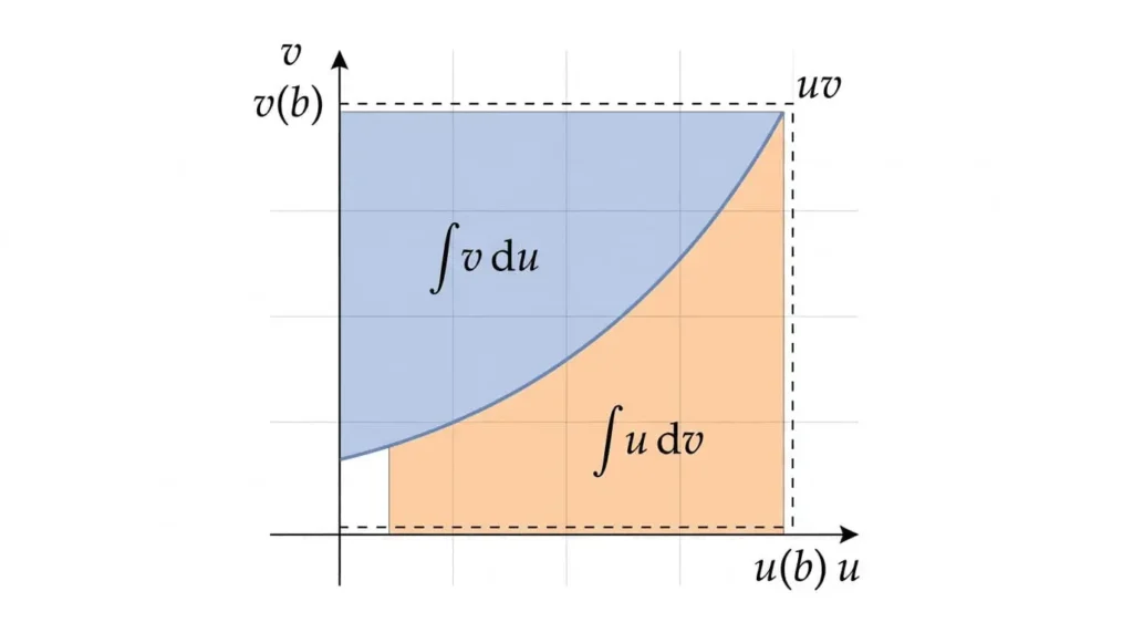
In the diagram above, the horizontal axis represents values of \(u\) and the vertical axis represents values of \(v\). The curve traces the path of the point \((u(x), v(x))\) as \(x\) varies. The total area of the surrounding rectangle is \(u \cdot v\). This area is shared between two complementary regions: the horizontal strip (\(\int v\, du\)) and the vertical strip (\(\int u\, dv\)). The equation \(\int u\, dv = uv – \int v\, du\) is simply the statement that these two regions add up to the rectangle — nothing more, nothing less.
This geometric perspective connects integration by parts to broader ideas in multivariable calculus and even to Green’s theorem in two dimensions, making it a conceptual cornerstone for students progressing to university-level analysis. If you are building toward that level of understanding, our introduction to the Fundamental Theorem of Calculus provides the essential bridge.
Key Properties and Special Cases
The core formula generates several useful results that appear so frequently they are worth knowing by name.
Reduction Formulas
When an integrand contains a power \(x^n\) paired with a trigonometric or exponential function, repeated integration by parts produces a reduction formula — a recursive relationship that reduces the power by one at each step. For example:
\int x^n e^x \, dx = x^n e^x – n \int x^{n-1} e^x \, dx
\]
Applying this reduction \(n\) times eventually brings the exponent down to zero, leaving \(\int e^x dx = e^x + C\), which can be written immediately. Reduction formulas are especially prominent in university calculus courses and form the theoretical basis of the tabular method.
Integration by Parts for Definite Integrals
The definite integral version evaluates boundary terms directly and requires no separate constant of integration:
\int_a^b u \, dv = \bigl[u(x)\,v(x)\bigr]_a^b – \int_a^b v \, du
\]
The key point is that you must evaluate \(u(x)v(x)\) at both limits before proceeding — it is not enough to find the indefinite integral and evaluate at the end.
Conclusion: Mastering Integration by Parts
Integration by parts is not just a formula to memorise — it is a way of thinking. It tells you that a seemingly impossible integral can be converted into a manageable one by making a clever trade: differentiate one factor to simplify it, integrate the other to absorb it, and account for the exchange through the boundary term \(uv\). The technique begins with the product rule of differentiation, lives through the LIATE rule and the tabular method, and reveals itself geometrically as the partitioning of a rectangle into complementary areas.
Whether you are sitting an A-Level paper, the AP Calculus BC exam, an IB Higher Level assessment, or a first-year university examination, integration by parts will appear — and it will reward students who understand it deeply rather than those who have merely memorised the formula. Practice the three core example types (polynomial × trig, logarithm alone, and cyclic exponential × trig) until each feels completely routine. From there, reduction formulas and the tabular method will become natural extensions rather than new hurdles.
Ready to test yourself? Our integration by parts practice problems offers graded exercises — from basic to A-Level and AP Calculus BC standard — each with a full worked solution and a hint to guide you without spoiling the answer.
For an authoritative reference, the Wikipedia article on integration by parts provides additional mathematical generalisations including the Riemann–Stieltjes and Lebesgue–Stieltjes forms for those progressing to graduate-level analysis.